Long-run equilibrium in time series cointegration
“Long-run equilibrium” in the context of cointegration means:
Even though individual time series (e.g., prices, GDP, exchange rates) may drift or trend over time, a certain linear combination of them remains stable over the long term.
🧠 More concretely:
- Suppose you have two nonstationary time series:
- t: house prices
- Xt: construction costs
- Both might trend upward over time. But if they are cointegrated, then the difference or some linear combination like: Yt−βXt is stationary—meaning it fluctuates around a constant mean.
That implies:
While Yt and Xt may each wander on their own, they do so in a way that keeps their gap stable over time.
🧭 Interpretation:
In economic terms, cointegration suggests there’s a “gravitational pull” between variables—whenever they drift apart, market forces (or economic logic) pull them back together.
This equilibrium doesn’t mean the series are flat or fixed, but that their relationship is stable, despite individual trends.
Example
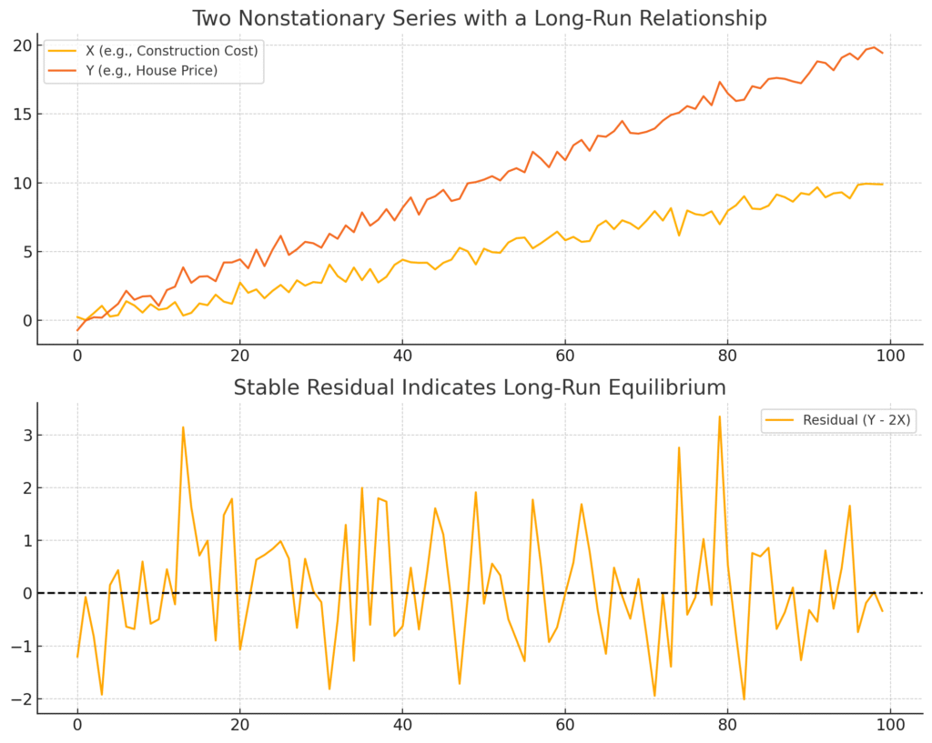
The visualization shows what a long-run equilibrium looks like in cointegration:
- Top Plot:
- Two nonstationary time series (X and Y) trend upward.
- Y is roughly double X, so they drift together.
- Bottom Plot:
- The difference (Y − 2X), or the “residual,” fluctuates around a constant mean, which implies a stationary linear combination.
- This stability in the residuals is what defines a cointegrated relationship — the essence of long-run equilibrium.